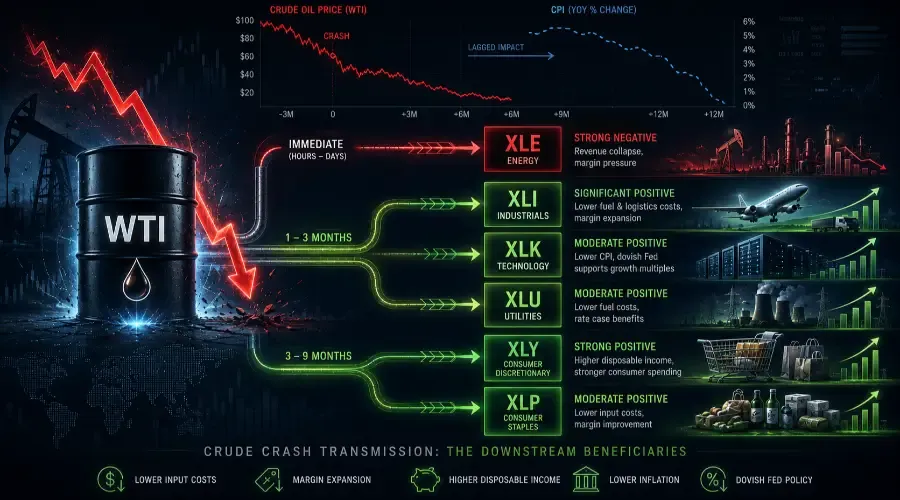
A $920 million crude oil short was placed seventy minutes before prices collapsed – and by the time the news hit financial feeds, the sector rotation was already underway. Oil price crashes don't announce themselves politely. They arrive through a combination of demand signals, OPEC decisions, and positioning unwinds – and they trigger a twelve-sector repricing sequence that runs for two to three quarters after the headline event. Most traders watch XLE fall and stop there. But the real trade is in the sectors that haven't moved yet and will – predictably, mechanically, and with documented historical precedent. This is the full crude oil crash trading strategy: the sector winners, the transmission chain, and the timing windows that let you position ahead of the crowd.

Why This Matters More Than Most Traders Realize

An oil price crash is the most underappreciated positive macro catalyst in markets. While the financial media focuses on the losers – energy company layoffs, rig shutdowns, regional bank stress in oil-producing states – the crash is simultaneously delivering a broad-based input cost reduction across the rest of the economy. Every sector that uses energy, transport, or petrochemical-derived inputs sees its cost structure improve. That is most of the S&P 500. When you step back and look at how falling oil prices impact stocks, you quickly realize the story goes far deeper than XLE.

The historical numbers are striking. A 30% sustained decline in crude oil has historically added 0.4–0.7 percentage points to operating margins for US airlines within two quarters. Consumer staples producers see packaging and logistics costs fall. Retailers see transport costs compress. Utilities burning oil or natural gas see generation cost relief. The Federal Reserve sees lower headline CPI, which gives it room to hold or cut rates – a tailwind for rate-sensitive sectors.

What most competing analysis misses entirely is the distinction between a demand-driven crash and a supply-driven crash. These two causes produce the same XLE decline but very different downstream sector outcomes. A supply-driven crash (OPEC production war) is unambiguously positive for most of the economy – costs fall while demand stays intact. A demand-driven crash (global recession signal) means costs fall but the revenue side is also under pressure. Knowing which type you are dealing with is the single most important analytical step, and it determines whether you aggressively rotate into the beneficiaries or tread more carefully. [LINK: Energy Hub]

The Chain Reaction: How a Crude Crash Moves Through the Economy

The first sector to move is always Energy (XLE), and it moves before you finish reading the headline. When crude oil falls sharply, the revenue models of every exploration and production company, integrated major, and oil services firm reprice in real time. The futures market is instantaneous. XLE can fall 5–8% in a single session on a major crash, and unlike the upstream positive from a spike, there is no buffer here – lower prices mean lower revenue, period. Producers with high breakeven costs face the steepest damage; those with sub 40 break-even barrels can weather a sustained decline;those with 55–65 breakeven costs face existential stress in a prolonged downturn.

The second movement – the one that separates this analysis from what you find in generic financial content – begins immediately but takes weeks to fully show up in prices. Materials (XLB) faces a mixed signal. Fertiliser companies within XLB see natural gas and petrochemical input costs decline, partially improving their margins. But mining companies see lower energy costs for extraction operations – a net positive for margins. The commodity correlation that lifted XLB during a crude spike now works in reverse for energy-correlated names, but energy-consuming industrials within the materials space see genuine cost relief. The crude oil crash transmission chain explained this way reveals a much more nuanced picture than what you'll find in surface-level commentary.

The third movement is where the real institutional opportunity lives. The supply chain absorption layer – Industrials (XLI) – begins repricing within the first four weeks. Airlines are the most dramatic example: jet fuel typically represents 20–25% of their operating cost base, and a 30% decline in crude translates to hundreds of millions in annualised savings for a major carrier before a single hedging contract expires. Trucking and logistics companies see diesel costs fall, improving per-mile economics almost immediately. The important nuance is timing: if the airline or trucking company hedged fuel costs at higher prices, the benefit shows up in cash costs but not in P&L until the hedges roll off – typically one to four quarters depending on the hedging program.

Utilities (XLU) see genuine cost relief from falling oil and natural gas prices. Regulated utilities cannot immediately pass savings to ratepayers – that process moves slowly through state regulatory commissions – but their operating cash flows improve, and rate cases filed for the next regulatory cycle reflect lower assumed fuel costs. The long-term credit profile of fuel-intensive utilities improves. Technology (XLK) benefits through the Fed policy channel: lower crude means lower CPI, which gives the Federal Reserve room to hold or ease rates, which reduces the discount rate applied to long-duration growth stocks. This is a second-order benefit but historically a meaningful one – in the 2014–2016 oil crash cycle, the Fed's ability to stay accommodative despite global uncertainty was directly linked to the absence of energy-driven inflation.

The final movement reaches the consumer layer in the three-to-nine-month window, and this is where the crash becomes a genuine economic positive. Consumer Discretionary (XLY) benefits from rising disposable income as fuel costs fall – every dollar reduction in what you spend at the gas pump is a dollar available for discretionary spending. Consumer Staples (XLP) sees input cost relief across packaging, logistics, and commodity-linked ingredients, expanding margins without requiring price increases. The compounding effect – lower input costs plus steady or rising consumer demand – makes the six-to-nine-month period following a supply-driven crash one of the most reliably positive windows for consumer and industrial sector performance.

Sector-by-Sector Impact: Who Wins, Who Loses, and When

Energy (XLE) – Strong Negative – Immediate.

XLE is the direct and unavoidable victim. Revenue falls immediately, capex programs get suspended, dividend cuts follow if the crash is sustained, and oil services companies within the sector face order cancellations. The magnitude of XLE damage scales with the severity and duration of the crash: a 20% decline in crude for six weeks is painful but manageable; a 50% decline sustained for twelve months, as in 2014–2016, produces XLE declines of 40%+ from peak. The trap is buying XLE on the initial dip – the bottom in crude oil prices typically comes months after the initial crash, as supply takes time to adjust downward.

Materials (XLB) – Mild Negative to Neutral – Immediate.

Materials presents the most nuanced signal in a crude crash. Energy-correlated commodity names (natural gas liquids, petrochemicals) fall with crude. But fertiliser producers see input cost relief (natural gas is a primary feedstock for nitrogen fertiliser), and mining companies see lower energy costs for extraction. The net XLB signal is close to flat in a supply-driven crash, and mildly negative in a demand-driven crash where global industrial activity is also falling. Watch the XLB sub-components rather than the ETF headline number.

Industrials (XLI) – Significant Positive – 1–3 Months.

This is the first major winner and the trade most retail traders undersize. Airlines, truckers, and logistics companies within XLI see their largest input cost decline in the fuel line. In practice, airline stocks benefit from oil crashes almost mechanically – fuel is their single biggest variable cost. Airlines report the benefit within one to two quarters; freight companies see margin expansion as diesel falls. Defence and aerospace names within XLI are largely neutral – their fuel exposure is indirect and contracts are multi-year. The cleanest trade within XLI is in the transport sub-sector: airlines, trucking, and package delivery companies. Expect XLI transport names to outperform the broader index by 5–10% over two quarters following a sustained 30%+ crash.

Utilities (XLU) – Moderate Positive – 1–3 Months.

Lower fuel costs improve the operating economics of fuel-dependent utilities, and the Fed policy implication of lower inflation is a direct positive for bond-proxy sectors like XLU. Rate-regulated utilities see their next rate cases filed at lower assumed fuel costs, improving long-term earnings visibility. Expect XLU to outperform SPY by 2–4% over two to three quarters following a sustained crash – not a dramatic move, but a reliable one.

Real Estate (XLRE) – Moderate Positive – 1–3 Months.

The mechanism runs through the interest rate channel. Lower crude reduces inflation expectations, which reduces upward pressure on the 10-year Treasury yield, which improves the relative valuation of yield-competing assets like real estate investment trusts. This is not a direct energy cost benefit but a financial conditions benefit. XLRE historically outperforms in the six months following a sustained crude crash when the demand-driven vs supply-driven distinction favours the former narrative – lower oil + stable economy = lower rates + strong property demand.

Technology (XLK) – Moderate Positive – 1–3 Months.

The Fed policy channel delivers the benefit to XLK. Lower crude → lower CPI → Fed holds or cuts → lower discount rate → growth stock multiple expansion. Data center energy costs also decline modestly. The XLK benefit is real but second-order – it depends on the Fed actually responding to lower energy prices, which happens more reliably in supply-driven crashes than demand-driven ones where recession risk clouds the outlook. In a clean supply-driven crash, expect XLK to outperform by 2–4% over two quarters.

Consumer Discretionary (XLY) – Strong Positive – 3–9 Months.

This is the largest lagged winner and the trade with the longest time horizon. Falling gasoline prices restore disposable income – the income effect on consumer spending is direct and meaningful. A 50-cent decline in national average gasoline prices is worth roughly $70 billion in annualised consumer purchasing power across the US economy. That money flows into restaurant spending, travel, retail, and entertainment – all of which are heavily represented in XLY. The lag is three to six months because the income effect takes time to accumulate and because consumer confidence adjusts slowly. Historically, XLY outperforms SPY by 6–10% in the two to three quarters following a major supply-driven crude crash.

Consumer Staples (XLP) – Moderate Positive – 3–9 Months.

Input cost relief on packaging (plastics, cardboard), transport (logistics), and energy-linked commodity ingredients expands margins without requiring price increases. XLP companies – food producers, household goods manufacturers, beverage companies – benefit from the cost side while the demand side remains stable. The margin expansion shows up in the next one to two earnings cycles after the crash. Historically, XLP outperforms by 3–5% over two to three quarters following a sustained decline.

Communication Services (XLC) – Mild Positive – 3–9 Months.

As consumer disposable income rises and corporate margins recover across the economy, advertising budgets tend to expand. XLC's advertising-dependent revenue base benefits from this second-order consumer confidence recovery. The effect is modest and lagged – expect 1–2% outperformance relative to SPY in the two to three quarters following a major crash, primarily from the digital advertising names within the sector.

Healthcare (XLV) – Mild Positive – 3–9 Months.

Device manufacturing costs, pharmaceutical supply chain logistics, and facility energy operating costs all decline with crude. The bigger benefit to XLV is the removal of inflationary pressure that might otherwise trigger a Fed response hostile to growth multiples. In a supply-driven crash, XLV is a mild positive that underperforms the cyclical beneficiaries but outperforms a stable baseline. Expect modest 1–2% relative outperformance over two to three quarters.

Financials (XLF) – Mixed – 1–3 Months.

Financials connect all three layers and face genuinely competing forces in a crude crash. On the negative side: regional banks with energy loan portfolios face rising credit losses as E&P companies struggle, oil-producing region real estate faces valuation pressure, and energy-related corporate bonds deteriorate. On the positive side: lower inflation reduces the probability of a hawkish Fed, steeper yield curves become possible, and consumer credit quality improves as discretionary income rises. The net signal depends heavily on whether the crash is supply-driven (net slightly positive for XLF) or demand-driven (net negative as broader credit risk rises). Watch regional bank stocks with disclosed energy loan concentrations – they are the tell for which direction XLF resolves.

Historical Cases That Confirm the Pattern

1998–1999 | Asian Crisis Demand Collapse – Crude Falls Below $11

The Asian financial crisis crushed global industrial demand, sending WTI crude below $11 per barrel by the end of 1998 – a collapse of nearly 60% from its 1996 highs. This was a demand-driven crash, which meant the sector rotation was more complex than a clean supply-driven event. XLE fell sharply and took two years to recover meaningful ground. However, US domestic consumer sectors – insulated from the Asian demand collapse – benefited from the input cost relief. Airlines reported margin improvements in 1999 as jet fuel costs declined. The lesson this case teaches is the demand-driven distinction: US consumer beneficiaries still won, but the scale was more modest because global growth concerns offset some of the income effect. Lag window: XLE fell immediately and stayed down; XLI domestic transport names improved within two quarters; XLY consumer improvement within three to four quarters.

2014–2016 | OPEC Production War – The Definitive Supply-Driven Crash

This is the cleanest modern case study for a supply-driven crude crash. OPEC's November 2014 decision to maintain production despite falling prices sent WTI from 100 per barrel to a low of 26 by February 2016 – a 74% decline over fifteen months. XLE lost over 40% of its value, and energy-related high-yield bonds faced a wave of defaults. But the mirror image played out exactly as the model predicts: airlines reported record profits in 2015 and 2016 as jet fuel costs collapsed. Delta Air Lines alone saw its fuel bill decline by over 2 billion in 2015.US consumer spending held steady and then improved as gasoline fell below 2 per gallon nationally. XLP food companies saw input cost relief improve margins by 50–100 basis points. The Federal Reserve cited lower energy prices as a factor allowing it to move slowly on rate normalisation. Every layer of the downstream sector benefited – precisely because the crash was supply-driven, not a demand signal. Lag window: XLE immediate 40%+ decline; XLI airlines within two quarters; XLY and XLP within three to four quarters; Fed accommodativeness sustained throughout.

2025–2026 | The Short-Driven Crash and the Market's Initial Confusion

The $920 million crude oil short placed seventy minutes before prices collapsed in early 2025 – documented by the Economic Times and covered by the BBC – illustrated a modern dynamic: the crash arrived faster than the sector rotation playbook could activate. Markets initially struggled to distinguish between a demand-signal crash and a positioning-driven crash. The EIA data confirmed in the subsequent weeks that US crude inventories were building – a supply signal, not a demand collapse. Stocks in the initial aftermath fell more than 1% broadly as the market processed the signal before ultimately recovering as the supply-driven interpretation took hold. Transport names within XLI began outperforming within four to six weeks as the fuel cost benefit became clear in forward guidance. Lag window: initial broad market confusion cleared within two to four weeks; XLI transport benefit within one quarter; consumer sector benefits tracking into following quarters.

The Before/During/After Playbook

Before: What to Watch for Early Warning

Monitor OPEC+ meeting calendars and Saudi Aramco production announcements (published by OPEC's monthly oil market report, available free at opec.org). The most reliable pre-crash signal for supply-driven collapses is a pattern of OPEC members publicly debating production quotas – which signals internal cohesion is breaking down. When Saudi Arabia signals it will defend market share over price, the supply-driven crash setup is in place. This discussion always surfaces in the oil market report two to three months before the actual price move.

Watch US crude oil inventory data, published every Wednesday at 10:30am EST by the EIA (eia.gov/petroleum). Consecutive weekly inventory builds of three million barrels or more – especially during periods of seasonal demand strength – signal supply is outpacing demand. Four to six consecutive build weeks is historically the pre-crash accumulation pattern. This indicator led the 2014 crash by approximately eight weeks.

Track the spread between WTI and Brent crude (available in real time on CME and Bloomberg). A narrowing Brent-WTI spread signals US supply is catching up with global benchmarks – a bearish signal for domestic producers and a leading indicator that the global price floor is weakening. When Brent and WTI converge within $2 per barrel during a period of rising US production, the setup for a supply-driven crash is maturing.

During: Positioning When the Crash Is Live

Underweight or exit XLE immediately on confirmation of a sustained move below a key technical level – not on the first day of a single-session decline. The one-day crash in crude is often a positioning unwind that partially reverses. The confirmation signal is a second weekly close below the prior range low. Once that confirmation is in, reduce XLE exposure and do not attempt to catch the falling knife – the bottom in crude oil prices typically arrives six to twelve months after the initial crash, not six to twelve days.

Initiate a long position in XLI transport names via the iShares Transportation Average ETF (IYT) or selectively in airline stocks within XLI. Size this position for the one to two quarter time horizon, not a day trade. The fuel cost benefit takes one to two quarterly earnings cycles to appear fully in reported numbers – but the forward guidance language changes faster. Listen for airline management teams to say "we expect fuel savings to materialise in the next two to three quarters" – that is the signal the trade is on but not yet priced.

Rotate from XLE into XLY within your energy and consumer allocation. The XLE-to-XLY rotation is the core pair trade for a supply-driven crude crash and has historically delivered 8–12% relative performance over two to three quarters in cycles like 2014–2016. You are not making a direction call on the consumer – you are positioning for the mechanical income effect that falling fuel prices deliver to discretionary spending.

After: The Lagged Rotation Trade

Add XLP on earnings weakness in the first quarter after the crash, when food and staples companies are still reporting elevated prior-period input costs. The stock typically trades down on the backward-looking earnings miss while the forward-looking cost improvement is already locked in through commodity contracts. That gap between backward earnings and forward economics is your entry window. Expect XLP margin recovery to appear fully within two quarterly earnings cycles post-crash.

Monitor the Baker Hughes rig count weekly (rigcount.bakerhughes.com, published every Friday). When the rig count falls for eight to twelve consecutive weeks following a crash, US supply is genuinely contracting – and the stage is being set for the eventual price recovery that ends the crash trade. Begin reducing XLI transport exposure and rebuilding modest XLE exposure when the rig count shows its first three-week plateau, suggesting the supply contraction is maturing.

Watch for the first CPI print showing negative energy contribution (BLS data, second week of each month). When energy makes a negative contribution to headline CPI, the market begins pricing in a more dovish Fed – which lifts XLRE and XLU alongside the consumer sector recovery already underway. This confirms the full downstream rotation has transmitted and signals the beginning of the recovery phase for previously damaged rate-sensitive sectors.

The 3 Mistakes Most Retail Traders Make

Mistake 1: Buying XLE on the First Day of the Crash

The single most common and most costly mistake is treating the first day of a crude crash as a buying opportunity in XLE. The logic sounds reasonable: "Energy stocks have fallen 8% – they must be cheap now." The institutional reality is different. Major crude oil crashes – the ones that produce meaningful downstream sector rotation – do not bottom in days. They bottom in months. The 2014–2016 crash took fifteen months to find its floor. The 1998 crash took over a year. Buying XLE on day one of a crash that ultimately runs for twelve months means you are catching a falling knife with 40% of the decline still ahead of you. The correct approach is to wait for the EIA inventory data to show consecutive weekly draws – confirming supply is contracting – before rebuilding XLE exposure.

Mistake 2: Missing the Demand-Driven vs Supply-Driven Distinction

The second mistake is treating every crude crash identically. A trader who correctly sized an XLY long in the 2014–2016 supply-driven crash would have been rewarded. A trader who applied the same playbook to the 2008 demand-driven crash – where crude fell because global industrial activity was collapsing – would have found that XLY was also falling, because the income effect was overwhelmed by unemployment and credit stress. Before executing any downstream sector rotation trade following a crude crash, you need to answer one question: is crude falling because supply is too high, or because demand is too low? Supply crash: execute the full downstream beneficiary playbook. Demand crash: be selective, focus on cost-benefit names rather than income-effect names, and size positions smaller.

Mistake 3: Ignoring the Energy Loan Exposure in Regional Banks

The third mistake is overlooking XLF's energy credit exposure. Regional banks in Texas, Oklahoma, North Dakota, and other oil-producing states carry significant energy loan portfolios. When crude crashes and E&P companies face cash flow stress, loan loss provisions rise, and regional bank stocks within XLF underperform the broader financials sector by a wide margin. In the 2015–2016 cycle, energy-exposed regional banks fell 20–35% while large-cap money-centre banks with diversified loan books held up significantly better. If you are rotating into XLF during a crude crash – because the rate environment is benign – make sure you are accessing the large-cap diversified bank exposure, not the regional bank energy exposure that is being hit from the opposite direction.

Bottom Line: The One-Sentence Institutional Framework

When crude oil crashes on supply dynamics – not demand collapse – sell XLE, buy XLI transport names within one quarter, rotate from XLE to XLY within two quarters, and use XLP margin recovery as the three-quarter confirmation that the full downstream chain has transmitted.

This framework works across cycles because the underlying mechanics – input cost reduction flowing through every energy-consuming sector in a documented sequence – do not change between 1998 and 2026. The headlines change. The geopolitical triggers change. The specific companies that win and lose change. The chain does not.

The retail edge is not knowing that crude fell. It is knowing that the airline margin recovery, the consumer income effect, and the XLP cost relief are all coming – just on a timeline measured in quarters, not days. Most market participants stop thinking about the crude crash after XLE makes the front page. The real alpha is two to three quarters away, in sectors most people never connected to a barrel of oil.

Run this scenario through the [Breakout Bulletin Ripple Engine](LINK: Ripple Engine Tool) to see the full sector transmission map, set intensity to match the magnitude of the crash you are analysing, and get the complete sequence of downstream beneficiaries with timing windows for all twelve sectors.

FAQ: Crude Oil Price Crashes and Stock Market Impact

What happens when crude oil prices crash?

When crude oil prices crash, energy stocks usually fall first, while airlines, transportation companies, consumer discretionary stocks, and many industrial sectors often benefit later from lower fuel and input costs.

Which sectors benefit most from falling oil prices?

Airlines, transportation companies, consumer discretionary stocks, and industrial sectors often benefit the most because lower fuel and logistics costs improve profit margins and consumer spending power.

Which sectors perform poorly during an oil price crash?

Energy companies, oil producers, oil services firms, and energy-heavy regional banks usually perform poorly because falling crude prices reduce revenues, profitability, and energy sector investment.

How do falling oil prices affect inflation?

Lower oil prices reduce transportation, manufacturing, logistics, and energy costs across the economy, which can lower inflation pressure over the following quarters.

Why do airline stocks benefit when oil prices fall?

Fuel is one of the largest operating expenses for airlines. Lower crude oil prices reduce jet fuel costs, which can significantly improve airline profit margins.

How does the Federal Reserve react to oil price crashes?

If falling oil prices reduce inflation significantly, the Federal Reserve may adopt a more accommodative stance by slowing rate hikes or considering rate cuts.

What is the difference between a supply-driven and demand-driven oil crash?

A supply-driven oil crash happens when oil production rises faster than demand, which is generally positive for consumers and businesses. A demand-driven crash occurs during economic slowdowns, where falling demand signals broader economic weakness.

What is the typical sector rotation during an oil crash?

The usual sequence starts with Energy (XLE) underperforming first, followed by strength in Industrials (XLI), Consumer Discretionary (XLY), Consumer Staples (XLP), and rate-sensitive sectors as inflation pressures ease.

This post is part of the BreakoutBulletin "What Happens When" series. [LINK: Energy Hub] · [LINK: Series Pillar Page]

Educational content only. Not investment advice. Past sector performance patterns do not guarantee future results.