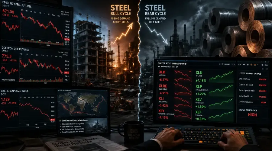
What Happens When Steel and Iron Ore Prices Drop

Iron ore prices on Chinese exchanges and global hot-rolled coil steel benchmarks tracked by commodity pricing services are among the most actively followed industrial indicators in institutional trading desks – yet they are almost completely absent from retail trader analysis. When iron ore collapses 30% in three months, as it did in 2021 when Chinese property developer stress first became visible, the signal is not about steel. It is about the largest construction market on earth grinding to a halt. When US hot-rolled coil steel futures fall through multi-year support, it is not about metal. It is about auto manufacturers cutting production schedules and infrastructure spending stalling. The traders who read these prices as commodity news miss the entire point. The traders who read them as forward economic signals have a six to twelve week head start on the sectors that get hit.

Why This Matters More Than Most Traders Realize

Steel and iron ore together form the backbone of physical economic activity in a way that no financial instrument can replicate. Steel goes into buildings, bridges, vehicles, appliances, industrial machinery, pipelines, and shipping containers. Iron ore is the raw material that feeds the global steel production system, with China accounting for approximately 70% of global seaborne iron ore demand and over 50% of global steel production. When these two prices fall together – particularly when Chinese iron ore demand is the driver – the signal is a forward read on construction activity, manufacturing investment, and durable goods production that arrives before any of it shows up in official economic data.

The key quantitative framing: approximately 50% of global steel consumption goes into construction and infrastructure, 17% into automotive manufacturing, 16% into mechanical equipment, and the remaining 17% across energy, appliances, and packaging. A steel price crash meaning is not a single-sector story. It is a demand signal that runs simultaneously through real estate, automotive, industrial machinery, and energy infrastructure – four of the most economically significant investment categories in the global economy.

What competing analysis misses is the tariff distortion problem. US domestic steel prices – tracked by HRC hot-rolled coil futures on the CME – can behave very differently from global steel benchmarks because of Section 232 tariffs that have been in place since 2018. A US trader watching only domestic steel prices can get a completely misleading signal. The institutional approach watches both simultaneously and understands when the divergence is a tariff story versus a demand story. [LINK: Metals Hub]

What This Is Really Saying: The Forward-Looking Reframe

Unlike copper – which leads the economic cycle by six to nine months – steel and iron ore prices are better understood as coincident-to-early-lagging indicators that confirm a slowdown already beginning rather than predicting one that has not started. The distinction matters enormously for how you use the signal.

Copper falls when construction firms and manufacturers begin reducing forward order pipelines – before any projects are cancelled. Steel prices fall when the cancellations actually start happening and mills begin losing orders. Iron ore falls when Chinese steel mills reduce production because their order books are already emptying. This sequence means that if you are watching copper alongside steel and iron ore, you have a two-signal system: copper gives you the early warning, steel and iron ore give you the confirmation.

The most important analytical reframe is geographic. Iron ore and Chinese steel prices are primarily reading the health of China's construction and infrastructure investment cycle. US HRC steel futures are primarily reading the health of US automotive production and domestic construction activity. These two signals are related – Chinese industrial slowdowns eventually transmit globally – but they are not identical. An iron ore collapse driven by Chinese real estate developer stress does not automatically produce a US automotive steel demand decline in the same quarter. Identifying which signal you are looking at – China-driven or US-driven – determines which US equity sectors you rotate in response to.

The practical forward-looking reframe: when iron ore and Chinese rebar prices fall together, you are seeing a signal about Chinese fixed asset investment that will appear in official Chinese GDP data one to two quarters later, in global commodity demand data one to three quarters later, and in US multinational earnings that depend on Chinese industrial activity two to four quarters later. Steel is not telling you what happened. It is telling you what the order books of the world's largest construction market look like right now.

The Lead/Lag Map: What Steel and Iron Ore Predict and When

0–4 weeks after a sustained steel and iron ore decline:

XLB Materials falls immediately as steel producers within the ETF – US Steel, Nucor, Steel Dynamics, commercial metals companies – see revenue estimates cut in real time. Chinese steel mill production data begins showing curtailments. Iron ore shipping rates (Baltic Capesize Index) fall as fewer bulk carriers are needed for ore transport.

1–3 months:

XLI Industrials faces growing headwinds as capital goods manufacturers, construction equipment producers, and industrial machinery companies begin seeing order intake fall. XLY Consumer Discretionary automotive sub-sector faces steel input cost changes that affect vehicle pricing dynamics – falling steel costs are a margin tailwind for automakers, but falling steel demand signals falling auto production volumes, which is a revenue headwind. XLRE Real Estate faces the clearest fundamental headwind as construction activity – the largest steel end market – contracts.

3–6 months:

The manufacturing slowdown signal begins appearing in official data: durable goods orders, ISM Manufacturing sub-indices for new orders, and industrial production readings. XLF Financials faces rising commercial real estate credit risk if the steel signal is confirmed by broader construction slowdown data.

6–12 months:

If the signal was a genuine demand collapse rather than a temporary price correction, equity markets broadly reflect the construction and manufacturing slowdown that steel prices announced six to twelve months earlier. The rotation from XLB and XLI into XLP and XLU is fully validated by this point.

Sector Rotation Sequence: Who Moves and In What Order

Materials (XLB) – Strong Negative – Immediate.

Steel producers within XLB are the direct and immediate victims of price declines. US Steel, Nucor, Steel Dynamics, and Commercial Metals Company all see earnings estimates revised lower as prices fall and volume signals deteriorate. The magnitude of XLB underperformance scales with the severity of the price decline – a 20% steel price drop historically produces 8–12% relative XLB underperformance over two quarters. Iron ore miners within XLB – or their international equivalents – also fall immediately as the demand signal validates.

Industrials (XLI) – Significant Negative – 1–3 Months.

Construction equipment manufacturers (Caterpillar, Deere within XLI), industrial machinery producers, and fabricated metal product companies all face falling demand when steel prices signal a construction and manufacturing slowdown. The key sub-sector to watch within XLI is the capital goods segment – these companies' order books are the first to reflect reduced construction and infrastructure investment plans. XLI underperforms by 4–7% over two quarters in a confirmed steel demand collapse scenario.

Consumer Discretionary (XLY) – Moderate Mixed – 1–3 Months.

The automotive sub-sector within XLY faces a counterintuitive split: falling steel input costs are a near-term margin tailwind for automakers, but falling steel prices signal falling auto production volumes ahead – because manufacturers only cut steel orders when they are reducing production schedules. The net XLY automotive signal from falling steel is mildly negative over two to three quarters, as the production volume decline overwhelms the input cost benefit. Home improvement retailers (Home Depot, Lowe's within XLY) face demand headwinds as construction activity contracts. Expect 3–5% relative underperformance over two quarters.

Real Estate (XLRE) – Significant Negative – 1–3 Months.

Construction is steel's largest end market globally, and a sustained steel demand collapse is one of the clearest leading signals for construction activity deceleration. XLRE faces a dual headwind: lower construction activity reduces the economics of new development, and the broader economic slowdown signalled by steel demand contraction raises recession risk for property valuations. Expect 4–6% relative underperformance over two quarters in a sustained steel demand decline.

Energy (XLE) – Moderate Negative – 1–3 Months.

Steel demand decline signals reduced pipeline construction, oil field infrastructure investment, and industrial energy consumption – all of which reduce energy sector capital expenditure and demand. The transmission is one quarter delayed, as energy companies adjust capex plans after seeing confirmed steel price signals in market data. Expect 3–4% relative underperformance over two quarters in a genuine industrial demand collapse scenario.

Financials (XLF) – Moderate Negative – 1–3 Months.

Commercial real estate lending faces increased risk when steel prices signal construction demand collapse. Regional banks with heavy commercial construction loan exposure – particularly in markets where development activity was strongest – face rising provisioning requirements as project economics deteriorate. Steel company credit quality also deteriorates with prices, affecting banks with industrial lending exposure. Expect 3–5% relative underperformance over two quarters, concentrated in regionally-exposed commercial lending banks.

Technology (XLK) – Mild Negative – 1–3 Months.

Enterprise capital expenditure softens when industrial activity contracts – reducing demand for manufacturing automation, industrial software, and B2B technology spending. The connection is second-order and slower than the direct industrial impact, but historically consistent. Data centre steel demand (structural steel for facilities) also provides a minor direct link. Expect 1–3% relative underperformance over two quarters.

Utilities (XLU) – Mild Positive Relative – 3–9 Months.

As the industrial slowdown signalled by steel prices validates in official economic data, defensive rotation into bond-proxy sectors begins. XLU benefits from both the recession-fear defensive premium and the Fed response – a confirmed construction and manufacturing slowdown increases the probability of rate holds or cuts, which re-rates bond-proxy utilities upward. Expect 3–5% relative outperformance over two to three quarters in a confirmed steel demand recession signal.

Consumer Staples (XLP) – Mild Positive Relative – 3–9 Months.

Defensive demand resilience makes XLP the standard rotation destination when construction and industrial signals validate a broader slowdown. Revenue resilience in food and household goods provides relative outperformance versus cyclicals without requiring absolute positive returns. Expect 2–4% relative outperformance over two to three quarters.

Healthcare (XLV) – Mild Positive Relative – 3–9 Months.

Inelastic healthcare demand provides defensive positioning benefit when steel signals validate a cyclical slowdown. The magnitude is modest – XLV's defensive premium is partially diluted by sector-specific policy risks that operate independently of the economic cycle. Expect 2–3% relative outperformance over two to three quarters.

Communication Services (XLC) – Mild Negative – 3–9 Months.

Corporate advertising budgets contract with industrial activity – when capital goods companies, automotive manufacturers, and construction firms reduce revenues, their marketing and communications spending follows. The lag is long and the magnitude is modest. Expect 1–2% relative underperformance over two to three quarters.

Historical Cases That Confirm the Pattern – Focus on the Early Signal

2015–2016 | Chinese Steel Oversupply Crisis and the Commodity Supercycle End

Chinese steel prices fell to multi-decade lows in 2015–2016 as Chinese mills – producing over 800 million tonnes of steel annually against actual demand of approximately 700 million tonnes – flooded global markets with excess supply. Iron ore fell below $40 per tonne, the lowest level since 2009. The global steel signal was reading two simultaneous problems: Chinese overcapacity depressing prices, and genuine global construction demand deceleration as the post-2009 infrastructure investment supercycle peaked. XLB fell over 25% from its 2014 highs by early 2016. XLI capital goods underperformed broadly as construction equipment manufacturers (Caterpillar reported falling machine sales in every quarter of 2015 and 2016). The early signal quality of this case was partially compromised by the overcapacity factor – US steel producers protected by tariffs (and later Section 232) performed better than global benchmarks suggested. This case established the tariff distortion problem that every subsequent analysis must account for. Lag window: XLB and global steel producers immediate; XLI capital goods within two quarters; Chinese fixed asset investment data confirmed three to four quarters after steel prices fell.

2018–2019 | Trade War Tariff Distortion – The False Domestic Signal

A trader watching only US HRC futures would have been long XLB while the global steel price was signalling the trade war demand disruption correctly. The subsequent collapse in US HRC prices in 2019 – as tariff-inflated inventories unwound – then sent a false collapse signal. This case directly motivates the dual-monitoring approach: US HRC alongside global HRC benchmarks (Argus, MEPS) and Chinese rebar futures. Lag window: US domestic steel disconnected from global signal throughout; global XLB equivalents signalled the trade disruption within two quarters; reconciliation occurred when US HRC fell in 2019.

2021–2022 | Evergrande and the Chinese Real Estate Signal

The collapse of China Evergrande Group – announced as a debt crisis in September 2021 – triggered the most significant Chinese real estate construction slowdown in modern history. Chinese iron ore prices fell over 50% from their May 2021 peak by November 2021 as steel mills began reducing production in response to collapsing real estate developer order books. This was arguably the most geographically specific major steel/iron ore signal in recent memory: the Chinese construction demand signal was real and severe, but US domestic steel prices remained relatively elevated through 2021 as domestic infrastructure spending (Infrastructure Investment and Jobs Act passing November 2021) offset the Chinese signal. The key lesson: iron ore falling on Chinese exchanges was a China-specific construction signal, not a global industrial signal – confirmed by the fact that US XLB steel producers outperformed Chinese equivalents significantly through 2021–2022. Traders who applied the full defensive rotation playbook based on iron ore alone missed the US-domestic offset. Lag window: Chinese iron ore immediate from May 2021; Chinese steel producers within weeks; US steel sector insulated through 2021; global XLI capital goods facing Chinese demand headwinds within two quarters.

The False Signal Trap: When to Ignore the Steel Decline

Steel and iron ore generate more false signals than copper because their prices are more susceptible to three specific distorting factors that have no equivalent in the copper market.

Tariff Distortion.

When US Section 232 tariffs are active, US domestic HRC steel prices can diverge substantially from global benchmarks. A US HRC decline may simply reflect tariff structure changes rather than genuine demand collapse. The filter: always cross-reference US HRC with global HRC benchmarks (Argus Media, MEPS International indices) and Chinese rebar futures. If global benchmarks are stable while US HRC falls, the signal is tariff-driven, not demand-driven.

Chinese Policy Stimulus Offset.

The Chinese government has historically responded to steel demand declines with infrastructure stimulus – announcing new rail, highway, or urban development projects that replace weakening private real estate demand. When iron ore falls but the Chinese government simultaneously announces large infrastructure packages, the steel demand signal may be partially offset within one to two quarters. The filter: monitor Chinese National Development and Reform Commission (NDRC) project approval announcements alongside iron ore prices. Rising NDRC approvals alongside falling iron ore signal that policy offset is coming.

Seasonal Inventory Cycles.

Steel prices routinely fall in Q4 as construction activity slows for winter in Northern Hemisphere markets and distributors reduce inventory ahead of year-end. A Q4 steel decline that reverses by March has almost no recession signal content. The filter: seasonal declines are typically 10–15% and recover fully within four to six months. Declines greater than 20% that persist through a full seasonal cycle – both winter and the subsequent spring construction season – carry genuine demand signal content.

The Confirmation Minimum Standard:

Before acting on a steel/iron ore decline signal, require at least two of the following: global benchmark confirmation (not just US HRC), Chinese iron ore declining in CNY terms (ruling out currency effects), ISM Manufacturing New Orders sub-index falling, and Baltic Capesize Index declining (fewer bulk carrier voyages means genuinely less ore moving).

The Trading Playbook

Before: What to Watch for Early Warning

Monitor CME hot-rolled coil steel futures alongside Argus or MEPS global HRC benchmarks weekly. The CME HRC contract (ticker HRC) provides real-time US domestic pricing. Argus Media and MEPS International publish weekly global HRC price indices covering European, Asian, and CIS markets. When both US and global benchmarks are declining together – not just one – the signal clears the tariff distortion filter and carries genuine demand information. A sustained break of more than 15% below the prior six-month average, held for four or more consecutive weeks across both US and global benchmarks, has historically preceded XLB and XLI underperformance with high reliability.

Track Chinese iron ore futures on the Dalian Commodity Exchange (DCE) – available in CNY per tonne terms on most major charting platforms and commodity data services. Chinese iron ore in CNY terms removes the currency translation effect and gives you the cleanest read on physical Chinese steel mill demand. When DCE iron ore falls more than 20% from a recent high over eight to twelve weeks, the signal is approaching confirmation threshold. Cross-reference with Chinese port iron ore inventory data (available from Bloomberg or S&P Global Commodity Insights, published weekly) – rising port inventories alongside falling prices confirms mills are reducing purchases.

Watch the Baltic Capesize Index weekly (published by the Baltic Exchange, available at balticexchange.com). Capesize vessels are the bulk carriers that transport iron ore from Australia and Brazil to Chinese steel mills. When the Capesize Index falls significantly – indicating fewer voyage bookings – it provides independent physical confirmation that iron ore shipments are genuinely declining. This is the hardest-to-fake confirmation in the steel signal toolkit, because it reflects actual vessel bookings rather than price quotes.

During: Positioning When Steel Is Breaking Down

Underweight XLB immediately when the dual US-global benchmark confirmation is in place. Within XLB, the steel producer sub-sector underperforms the broader materials index – reduce or eliminate Nucor, Steel Dynamics, and US Steel exposure while maintaining positions in less steel-sensitive XLB components like specialty chemicals if you wish to stay partially in the sector. The XLB underweight should be sized for a two to three quarter time horizon – steel price recoveries driven by China policy stimulus can be swift, so avoid open-ended shorts without defined exit criteria.

Reduce XLRE allocation below benchmark within two to four weeks of a confirmed steel demand breakdown signal, sized for a one to two quarter horizon. Real estate sector earnings are slower to reflect construction slowdown than XLB, giving you a window to reduce before the earnings impact appears. Use XLRE relative performance versus the broader market as your exit signal – when XLRE stops making new relative lows, the construction demand decline is likely bottoming.

Initiate a relative rotation from XLI into XLU, specifically targeting the capital goods and construction equipment sub-sector of XLI for reduction. Caterpillar and Deere within XLI are the most direct expressions of construction equipment demand – their relative performance to XLI broadly is your early confirmation that the steel signal is transmitting into equipment order books. When Caterpillar and Deere begin underperforming XLI, the signal has reached the industrial machinery layer and the XLI underweight is confirmed.

After: Reading the Recovery Signal

Watch Chinese rebar futures and DCE iron ore for a sustained three-week recovery above the breakdown level as the recovery signal. Chinese steel prices bottom before global steel prices and before any official economic data confirms the recovery – mirroring copper's role as the leading indicator on both the downside and the upside. When DCE iron ore recovers 15% from its trough and holds for three weeks, begin rebuilding XLB steel exposure and reducing the XLU defensive overweight.

Monitor Chinese construction starts data (National Bureau of Statistics monthly release) for the first sequential improvement after a period of year-over-year declines. Construction starts recovering – even modestly – is the earliest official data confirmation that the iron ore signal was accurate and is now resolving. Use this data point to size up the XLB and XLI recovery trade with more confidence.

Rebuild XLRE exposure when the 10-year Treasury yield stabilises or declines, confirming that the recession risk premium is fading from rate markets. XLRE's recovery from a steel-signalled construction slowdown historically begins one to two quarters after the Treasury yield peaks – giving you a rate market entry signal rather than relying on construction data alone.

The 3 Mistakes Most Retail Traders Make

Mistake 1: Watching Only US Domestic Steel Prices

The most structurally damaging mistake in steel market analysis is monitoring only CME HRC futures and concluding that US steel prices reflect global demand conditions. Since 2018, Section 232 tariffs have created a persistent premium in US domestic steel prices over global benchmarks that can be 100–300 per tonne wide. A US trader watching HRC can see prices rising while global steel demand is collapsing – missing the signal entirely. The institutional approach monitors both US HRC and global benchmarks simultaneously, treating the spread between them as a tariff premium indicator and requiring both to decline before acting on a demand signal. Any steel analysis that uses only one price series is incomplete by construction.

Mistake 2: Applying the Copper Lead Time to Steel

The second mistake is assuming steel signals carry the same six to nine month lead time as copper and positioning accordingly. Steel and iron ore are more coincident indicators – they confirm that order books are already emptying, not that they are about to. Acting on a steel decline as if you have six to nine months of lead time before sectors are affected means you are already late to the defensive rotation, not early. The correct framework treats copper as your early warning system and steel/iron ore as your confirmation signal – if both copper and steel are declining together, the recession signal is high-confidence and already underway, not predicted.

Mistake 3: Ignoring the Auto Sector Steel Signal

The third mistake is focusing exclusively on construction demand when interpreting steel price declines and missing the automotive manufacturing signal. Automotive steel demand represents approximately 17% of global steel consumption – significant enough that auto production cycle changes materially affect steel prices and vice versa. When auto manufacturers cut production schedules, their steel orders fall within weeks. Watching the monthly US auto sales data (seasonally adjusted annual rate, or SAAR, published first business day of each month by automotive manufacturers) alongside steel prices gives you the demand decomposition between construction-driven and automotive-driven declines. A steel decline accompanied by falling auto SAAR is a US-domestic demand signal; a steel decline with stable auto SAAR but falling Chinese iron ore is a China-construction signal. Each requires a different sector rotation response.

Bottom Line: The One-Sentence Institutional Framework

When US HRC steel futures and global benchmark prices both decline more than 15% from their recent six-month average, confirmed by falling DCE iron ore and a declining Baltic Capesize Index, sell XLB steel producers and XLRE immediately, reduce XLI capital goods within four weeks, and use Chinese iron ore futures recovering 15% from trough as the signal to reverse the rotation.

This framework works across cycles because the physical order-book mechanics of steel and iron ore procurement do not change between cycles. Construction contractors, steel distributors, and automotive manufacturers always reduce steel orders before they reduce production, before revenue falls, and before any official economic data reflects the change. The steel price is the order book made visible – it is the economic decision that was just made by thousands of procurement managers around the world, expressed as a single number on a trading screen.

The retail edge is using the dual-benchmark confirmation filter to avoid the false signals that destroy trading P&L, and understanding that steel is a confirmation tool, not a prediction tool – which means acting quickly when it confirms rather than waiting for additional evidence that arrives too late to be useful.

Run this scenario through the [Breakout Bulletin Ripple Engine](LINK: Ripple Engine Tool) to see how the steel and iron ore demand collapse transmission compares to the copper recession signal – the two together form the most reliable industrial demand warning system available to retail traders.

Frequently Asked Questions

What does it mean when steel prices fall?

Falling steel prices usually indicate slowing construction activity, weaker manufacturing demand, declining infrastructure spending, or reduced automobile production. It can act as an early economic slowdown signal.

Why are iron ore prices important?

Iron ore is the main raw material used to make steel. Since China consumes most global iron ore supply, falling iron ore prices often reflect weakening Chinese construction and industrial demand.

How do falling steel prices affect the stock market?

Steel price declines typically hurt cyclical sectors like Materials (XLB), Industrials (XLI), Real Estate (XLRE), and Energy (XLE), while defensive sectors like Utilities (XLU) and Consumer Staples (XLP) may outperform.

Are steel prices a recession indicator?

Steel prices are considered a coincident-to-early-lagging economic indicator. They often confirm that industrial demand and construction activity are already slowing.

What is HRC steel futures?

Hot Rolled Coil (HRC) futures track steel prices used in construction, automobiles, and manufacturing. Traders monitor them for industrial demand signals.

Why does China influence iron ore prices so much?

China accounts for over half of global steel production and consumes the majority of seaborne iron ore. Any slowdown in Chinese real estate or infrastructure directly impacts iron ore demand.

Which sectors suffer most when steel demand falls?

Materials, industrial machinery, real estate, construction equipment, and automotive-related companies usually face the biggest pressure during a steel demand decline.

This post is part of the BreakoutBulletin "What Happens When" series. [LINK: Metals Hub] · [LINK: Series Pillar Page]

Educational content only. Not investment advice. Past sector performance patterns do not guarantee future results.