
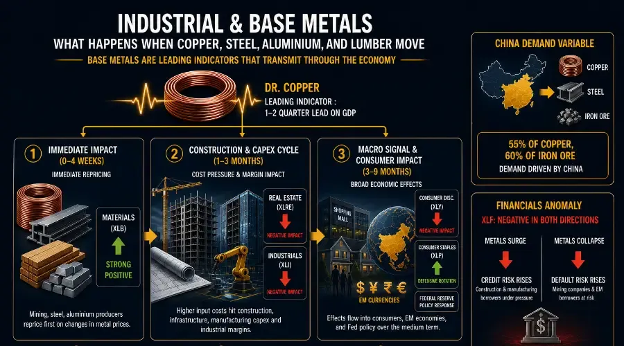
If energy is the economy's cost floor, industrial metals are its pulse. Copper wires every building, every motor, every grid upgrade on earth. Steel frames every bridge, every factory, every skyscraper. Lumber builds every home. When these materials move sharply, they are not just commodity stories – they are economic forecasts arriving before the official data does. For traders who understand base metals trading, these moves are some of the most reliable stock market indicators for economic health available.
Traders who understand base metals are not just trading commodities. They are reading the economy's forward calendar. This hub covers the three metal events that consistently generate the clearest sector signals: a copper price collapse, a steel and iron ore drop, and a lumber surge. Each tells a different story about where the economy is in its cycle – and each triggers a distinct, traceable chain of sector reactions.
Why Base Metals Are the Market's Most Reliable Leading Indicators
Every other market catalyst in this series reacts to something that has already happened – a Fed decision already announced, a jobs report already printed, a war already begun. Base metals are different. They price economic activity that has not yet shown up in the data.
This is why copper earned the nickname "Dr. Copper" – it has a PhD in economics. Copper demand is driven by construction, manufacturing, infrastructure spending, and consumer electronics production. These activities require copper months before the output they create shows up in GDP data or corporate earnings. When the global economy is genuinely accelerating, copper gets bought now so that factories can produce next quarter. When the economy is rolling over, copper orders get cancelled now – before the slowdown is visible in any official indicator.
The same logic applies to steel, iron ore, and lumber – they are ordered in advance of the construction and manufacturing activity that uses them. Their price movements are demand signals from the industries closest to real economic activity, arriving with a one-to-two quarter lead on the headline data.
This leading indicator quality is what makes base metal moves so valuable – and so dangerous to ignore. A sustained copper decline that the equity market is dismissing as a China-specific story has historically been one of the most reliable warning signs of broad economic deceleration. In 2008, copper peaked six months before the S&P 500 did. In 2011, copper's collapse from its April peak correctly forecast the global growth slowdown that hammered industrial stocks in Q3 and Q4 of that year.
The Metals Transmission Mechanism: How It Moves Through the Economy
Base metals transmit differently from energy. Energy flows downstream – from raw input to manufacturer to consumer. Metals transmit primarily through the construction and capital expenditure cycle, which means their impact concentrates in specific sectors rather than spreading evenly across all eleven. The key point is that industrial metals price action doesn't just tell you what already happened – it telegraphs what's coming.
Stage 1: Immediate Impact (0–4 Weeks)
Materials sector stocks (XLB) reprice immediately on a major metals move. Mining companies, steel producers, and specialty metals processors have revenues that move in near-direct proportion to spot commodity prices. Within XLB, names like Freeport-McMoRan (copper), Nucor (steel), and Alcoa (aluminium) are the first movers.
Simultaneously, the market reprices the companies most dependent on metals as inputs: heavy manufacturers, construction equipment makers, and auto producers (all within XLI). These businesses have multi-quarter hedging programs that delay the actual cost impact – but the market forward-prices the margin compression almost immediately.
What to watch in Stage 1: The XLB-to-XLI spread. If XLB rises sharply but XLI does not follow within two weeks, the market is pricing the metals move as a supply disruption (temporary) rather than a demand-driven surge (sustained). The distinction matters enormously for how far the downstream transmission will go.
Stage 2: Construction and Capex Cycle (1–3 Months)
This is where metals diverge most sharply from energy in their transmission path. The primary Stage 2 victims of a metals surge are not consumer-facing sectors – they are the capital-intensive industries that use metals to build things:
Real estate (XLRE): Construction costs are the most direct transmission channel. When steel and lumber surge simultaneously, the economics of new projects break down – developers delay starts, contractors revise bids upward, and housing affordability deteriorates. XLRE underperforms within one to two quarters of a sustained materials surge.
Industrials (XLI): Infrastructure and manufacturing capex projects get repriced or delayed. Capital equipment orders slow. Logistics companies face higher vehicle and maintenance costs. The industrial earnings cycle reflects metals costs with a one-quarter lag.
Technology (XLK): Less obvious but important – data center construction, semiconductor fab build-outs, and grid infrastructure for AI workloads all have significant copper and steel content. A sustained metals surge adds meaningful costs to the capex programs of hyperscalers and chip manufacturers. This is a newer transmission channel that has become increasingly relevant since 2020.
What to watch in Stage 2: Housing starts data (released monthly), ISM Manufacturing New Orders component, and corporate guidance from industrial companies on raw material costs. These three data series collectively show whether Stage 2 transmission is underway.
Stage 3: Broader Economic Signal (3–9 Months)
A sustained base metals decline – particularly copper – triggers Stage 3 effects that go beyond sector rotation into macro territory. When Dr. Copper is falling persistently, it is telling you that global manufacturing and construction activity is contracting. This eventually shows up in:
Emerging market currencies and equities: Chile, Peru, Zambia, and the Democratic Republic of Congo are large copper producers whose economies and currencies are directly correlated to copper prices. A sustained copper decline creates EM financial stress that can feedback into global risk appetite.
China-exposed equities globally: China accounts for approximately 55% of global copper consumption, 60% of iron ore demand, and 50% of steel production. When base metals fall on weak Chinese demand, every global company with significant China revenue faces a dual headwind – weaker demand and currency translation impact.
The credit cycle: Materials companies carry significant debt loads tied to commodity price assumptions. A sustained metals decline raises default risk in the mining sector and tightens credit availability for capital-intensive industries – adding a financial stress dimension to what began as a commodity price move.
Sector Reaction Map: Metals Surge vs. Metals Collapse
Materials (XLB) shows a ✅ Strong Positive impact during a metals surge, and a ❌ Strong Negative impact during a metals collapse, with the primary timing being Immediate.
Energy (XLE) shows a ✅ Moderate Positive impact during a metals surge, and a ❌ Moderate Negative impact during a metals collapse, with the primary timing being Immediate.
Industrials (XLI) shows a ❌ Negative impact during a metals surge, and a ✅ Positive impact during a metals collapse, with the primary timing being 1–3 Months.
Real Estate (XLRE) shows a ❌ Significant Negative impact during a metals surge, and a ✅ Significant Positive impact during a metals collapse, with the primary timing being 1–3 Months.
Technology (XLK) shows a ❌ Mild Negative impact during a metals surge, and a ✅ Mild Positive impact during a metals collapse, with the primary timing being 1–3 Months.
Utilities (XLU) shows a ❌ Mild Negative impact during a metals surge, and a ✅ Mild Positive impact during a metals collapse, with the primary timing being 1–3 Months.
Consumer Disc. (XLY) shows a ❌ Moderate Negative impact during a metals surge, and a ✅ Moderate Positive impact during a metals collapse, with the primary timing being 3–9 Months.
Consumer Staples (XLP) shows a ❌ Mild Negative impact during a metals surge, and a ✅ Mild Positive impact during a metals collapse, with the primary timing being 3–9 Months.
Comm. Services (XLC) shows a ❌ Mild Negative impact during a metals surge, and a ✅ Mild Positive impact during a metals collapse, with the primary timing being 3–9 Months.
Healthcare (XLV) shows a ➡️ Minimal Impact during a metals surge, and a ➡️ Minimal Impact during a metals collapse, with the primary timing being Lagged/Indirect.
Financials (XLF) shows a ❌ Negative (credit risk) impact during a metals surge, and a ❌ Negative (loan defaults) impact during a metals collapse, with the primary timing being 1–3 Months.
Key difference from the energy map: Financials are negative in both directions for metals. A metals surge raises credit risk for construction and manufacturing borrowers. A metals collapse raises default risk for mining companies and commodity-linked emerging market borrowers. The only scenario where XLF benefits from a metals move is a soft landing – a gentle metals decline that signals slowing but not collapsing growth, which is credit-positive for the broader loan book.
The China Variable: Why It Changes Every Calculation
No other commodity category is as dominated by a single buyer as industrial metals. China's share of global base metals demand is not a minor factor – it is the market. Any serious metals catalyst analysis requires a China demand assessment before the sector trade is built.
When a metals move is China-demand-driven:
The transmission is global and sustained. China's construction cycle (real estate + infrastructure) runs in multi-year waves. When Chinese steel and copper demand falls because property developers are defaulting (as in 2021–2023 with Evergrande and the broader property sector stress), the decline is structural and persistent – not a single quarter's worth of volatility. The sector rotation away from XLB and XLI needs to be sized as a multi-quarter position, not a quick trade.
When a metals move is supply-driven:
A mine strike in Chile, a refinery accident, a shipping disruption – these create sharp, short-lived spikes that rarely reach Stage 2 transmission. The market reprices XLB quickly but pulls back when supply normalizes. These are trading opportunities in the commodity and the materials sector, not macro rotation signals.
When a metals move is driven by a new demand theme:
The energy transition is creating a structural copper demand story that did not exist in previous cycles. Electric vehicles use four times the copper of internal combustion engine vehicles. Solar panels, wind turbines, and grid storage all have significant copper content. A copper surge driven by energy transition demand has different implications than a China infrastructure-driven surge – it is slower, more predictable, and more durable.
The critical question before any metals trade: Is China buying more or less? Is this supply or demand? Is this cyclical or structural?
Key Historical Metals Events and What They Produced
2020–2021: The Pandemic Reopening Metals Surge
Lumber prices rose 300% from their April 2020 lows to their May 2021 peak. Copper gained 50% from trough to peak over the same period. XLRE and XLI underperformed in the second half of 2021 as construction costs exploded and project economics deteriorated. Homebuilder stocks (within XLY) peaked in December 2020 – a full six months before lumber peaked – confirming that the equity market priced the construction cost headwind well before the commodity itself topped out. XLB was the top-performing sector in 2021.
2011: The China Demand Peak
Copper hit its all-time record of $4.60/lb in February 2011, driven by Chinese infrastructure spending. XLB gained 18% through mid-year. The subsequent collapse – copper fell 30% from its February peak to its December trough – was one of the cleanest leading indicators of the global growth slowdown that defined the second half of 2011. XLI margins compressed in Q3 and Q4 earnings. Consumer Staples (XLP) began outperforming as defensive rotation commenced – a textbook demand-shock reversal triggered by the copper signal.
2007–2008: Copper's Peak Six Months Before the Market
Copper peaked in May 2008 at 4.08/lb. The S&P 500 peaked in October 2007 – but XLB peaked in May 2008 alongside copper. The divergence between a resilient stock market and a deteriorating copper price through late 2007 and early 2008 was one of the clearest advance warnings of the GFC for traders watching the commodity. By December 2008, copper had fallen to 1.25/lb – a 69% collapse that confirmed the depth of the recession well before GDP data did.
2014–2016: Steel and Iron Ore Collapse
Chinese steel overcapacity combined with a global growth slowdown sent iron ore from 190/tonne to 38/tonne.
Bulk shipping companies collapsed. Brazilian and Australian mining equities fell 60–80%. The feedback into emerging market credit – particularly Brazilian and South African sovereign debt – created a multi-year EM bear market that ran in parallel with the metals decline. This is the case study for understanding how a metals collapse can cascade into a global financial stress event.
How to Trade Base Metals Catalyst Events: The Three-Phase Checklist
Use this checklist before, during, and after any major metals price move. One word of caution upfront: metals can gap violently on supply disruptions or China policy surprises – position size accordingly and respect the volatility.
Before a metals catalyst event:
Assess China PMI Manufacturing – specifically the new orders component, which is the most real-time copper demand signal available
Check LME copper warehouse inventories – rising inventories signal demand weakness; falling inventories signal genuine demand strength
Identify whether XLB move is broad (all metals) or narrow (single commodity) – broad moves carry macro implications; narrow moves are commodity-specific
Map your XLRE and XLI exposure: which holdings have the highest unhedged raw material cost exposure?
During the event:
Watch the XLB-to-XLI ratio – XLB outperforming XLI in a metals surge confirms the Stage 2 cost pressure is not yet priced in XLI
Monitor the Australian dollar (AUD/USD) – it is the highest-correlation currency proxy for Chinese metals demand; moves in AUD often lead XLB by days
Track EM currency performance alongside the metals move – widespread EM currency weakness alongside metals declines confirms China-demand-driven transmission
After the event (the lagged trades):
Set a one-quarter reminder to review XLRE and XLI earnings for construction cost and raw material cost commentary
Watch homebuilder guidance specifically – they are the most transparent reporters of lumber and steel cost impact
If copper is falling persistently, begin building a watchlist of defensive rotations into XLV and XLP as the potential Stage 3 macro signal plays out
Trading from outside the US? The metals transmission logic is global – use your local materials sector indices or commodity-linked ETFs; the chain reaction doesn't stop at borders
Three Metal Events Covered in This Hub
Each post below covers one specific metals catalyst with full Before / During / After trading analysis, sector reaction maps, and three or more historical case studies. What you'll notice is that each metal tells a slightly different story – copper reads the global economy, steel and iron ore track heavy construction, and lumber is uniquely domestic and housing-focused. Understanding those distinctions is what separates a precise sector trade from a blunt commodity bet.
→ What Happens When Copper Prices Fall (Recession Signal)
The most analytically rich metals post in the series. Covers the full Dr. Copper leading indicator framework, the distinction between China-demand-driven and supply-driven copper declines, the sector rotation playbook for a sustained copper bear market, and historical cases from 2008, 2011, and 2015. Also covers the false signal risk – when copper falls for reasons that do not predict recession, and how to tell the difference. [link]
→ What Happens When Steel and Iron Ore Prices Drop
Steel and iron ore are the construction economy's raw materials. Their decline signals stress in the building cycle – real estate development, infrastructure spending, and heavy manufacturing capex. Covers the China steel overcapacity dynamic, the impact on mining-dependent emerging market economies (Brazil, Australia, South Africa), and the XLRE and XLI rotation trade that typically follows a sustained iron ore decline. [link]
→ What Happens When Lumber Prices Surge
Lumber is the most domestically focused metals catalyst in the series – its price is driven primarily by US and Canadian housing demand and sawmill capacity, not global macro factors. Covers the homebuilder margin compression trade, the XLY sub-sector impact (Home Depot, Lowe's, homebuilders), the seasonal patterns that make Q1 the highest-risk period for lumber spikes, and the 2020–2021 case study where lumber's 300% surge was the single clearest signal of post-COVID construction sector stress. [link]
Continue Through the Catalyst Series
→ Pillar: The Complete Market Catalyst Framework
→ Hub 1: Energy Commodities – Oil, Gas, Uranium
→ Hub 3: Precious Metals – Gold, Silver, Platinum
→ Hub 4: Agricultural Commodities – Wheat, Corn, Soybeans
→ Hub 5: Macroeconomic Events – Fed, CPI, NFP, GDP
→ Hub 6: Central Bank & Policy – QE, Tapering, Tariffs, Tax
→ Hub 7: Geopolitical Events – Wars, Elections, OPEC, EM Crisis
All content on BreakoutBulletin is for educational purposes only and does not constitute financial advice or a recommendation to buy or sell any security.